Orthogonal Transformations
Wavelet
- DFT
DFT is the most important orthogonal transformation in signal analysis with vast
implication in every field of signal processing. The set of orthogonal (but not
normalized) complex sinusoids) is the family
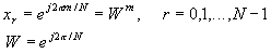
with the important property: 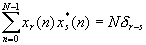
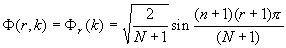
The conventional DFT is defined as:

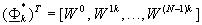
The corresponding matrices are
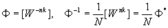
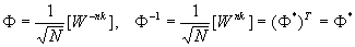
After normalization, the unitary DFT transformation matrix is
From a coding standpoint, a key property of DFT is that the basis vectors of the
unitary DFT (the columns of F *) are the
eigenvectors of a circulant matrix. That is, with the k column of F
* denoted by
 ,
,
we can show that F k* are the
eigenvectors in

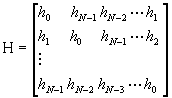
where H is any circulant matrix
In summary, we say that DFT transformation diagonalizes any circular matrix, and
therefore completely decorrelates any signal whose covariance matrix has the circulant
property of H.
- DCT
This transform is virtually the industry standard in image and speech transform coding
because it closely approximates the KLT especially for highly correlated signals, and
because there exist fast algorithms for its evaluation. The orthogonal set is:
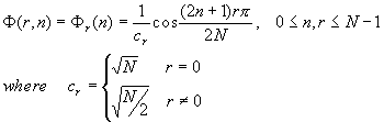
and F =[F (r,n)], F -1=F T
The basis vectors of DCT approach the eignvectors of the AR(1) process as the
correlation coefficient r ® 1. The
DCT is therefore near optimal (close to KLT) fot many correlated signals encountered in
practice. The characteristics of DCT are as follows:
- The DCT has excellent compaction properties for highly correlated signals.
- The basis vectors of DCT are eigenvectors of a symmetric tri-diagonal matrix:

whereas the covariance matrix of AR(1) process has the form
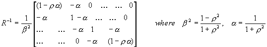
As r ® 1, we can see that b 2R-1® Q, which
confirms the decorrelation property.
- Discrete Sine Transform (DST)
This transform is suitable for signals with lower or negative correlation coefficient.
The unitary basis sequences are:
It turns out that the basis vectors of DST are eigenvectors of the symmetric
tri-diagonal Toeplitz (parallel diagonal elements are equal) matrix:
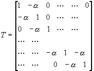
This matrix is somehow like the covariance matrix for AR(1) process with relative low |r |, say |r |<0.5. Of course for r =0, there is no benefit from transform coding since the signal is
already white, whereas the purpose is to transform the input signals to white signals,
i.e., ‘whiten’ the input signals.
- LOT
Orthonormal transform can be viewed as a special case of filter banks. A shortcoming of
above transforms is they split data stream block by block, thus after coding/compression,
the data may appear discontinuity at the bound of the adjacent blocks. Filter banks can be
used to conquer this shortcoming. LOT is also a special case of filter banks, which using
overlapped data block as input.
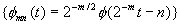
Wavelet
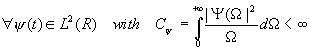
The wavelet transform (WT) is a mapping from L2(R) to L2(R) with
superior time-frequency localization.
- The continuous WT
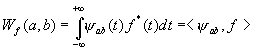
The continuous WT is defined as follows:
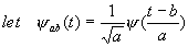
then the wavelet transform of f(t)Î L2(R) is the
inner product
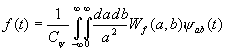
In the remainder of the letter, all time functions are assumed to be real. The invert
transform is then given by:
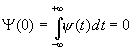
The admissibility condition Cy <¥
ensures that the continuous WT (CWT) is complete if Wf(a,b) is known for all a,
b. Furthermore the admissibility condition implies that DC gain Y
(0)=0, i.e.,
Thus, j (t) behaves as the impulse response of a bandpass
filter that decays at least as fast as |t|1-e . Of
course in practice it should be much faster to provide better time-localization.
The Parseval relation still holds for WT, i.e., within a scale factor, the WT is an
isometry from L2(R) to L2(R):

While it is possible to design wavelet to optimize, or tradeoff between time and
frequency resolutions, there is a fundamental limitation on what we can approach. This is
described by the uncertainty principle, which states that for any transform pair
f(t) and F(W ),

where 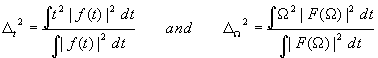
are measures of the variations (spread) of f(t) and F(W ).
We may consider 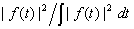 as the probability density function of random
variable t, then D 2t can be viewed as
the second moment of t. Actually an interpretation of above inequality, with D t and D W
as the effective duration and bandwidth of signal f(t), is: if a signal has bandwidth D W , then its duration must be longer
than 1/(2D W ) and vice versa. The
inequality holds for all transform in L2(R), including wavelet. Through the use
of different windows widths, wavelet transform can achieve arbitrarily small (at least
theoretically) D t and D W , although of course not both simultaneously.
as the probability density function of random
variable t, then D 2t can be viewed as
the second moment of t. Actually an interpretation of above inequality, with D t and D W
as the effective duration and bandwidth of signal f(t), is: if a signal has bandwidth D W , then its duration must be longer
than 1/(2D W ) and vice versa. The
inequality holds for all transform in L2(R), including wavelet. Through the use
of different windows widths, wavelet transform can achieve arbitrarily small (at least
theoretically) D t and D W , although of course not both simultaneously.
- The discrete WT
The CWT suffers from two drawbacks: redudancy and impracticality: the Wf(a,b)
is continuous for any a, b. we can try to sample the parameters (a, b) to obtain a set of
wavelet functions in discretized parameters.
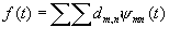
Let the sampling lattice be
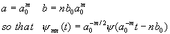
where m,n Î Z.
If this set is complete in L2(R) for some choice of f
(t), a, b, then the set {j mn(t)} are called affined
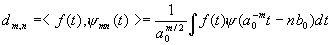
wavelets. Then we can express any f(t)Î L2(R) as
the superposition:
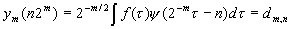
where the wavelet coefficient dm,n is the inner product
Such complete sets are called FRAMEs. They are not yet a BASIS. Frames do not satisfy
the Parseval theorem, and also the expansion using frames is not unique. In fact, it can
be shown that
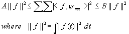
The family {j mn(t) } constitutes a frame if j (t) satisfies admissibility condition, and 0<A<B<¥ . Then the frame bounds are constrained by the following
inequalities
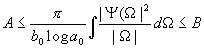
where 0<A £ B<¥ . The
condition holds for any choices of a0 and b0.
Next, if A=B=1, then the frame is call tight. But {j mn(t)
} is still not necessarily linearly independent. There still may be redundancy in this
frame. A frame is called exact if removal of a function leaves the frame incomplete.
Finally, a tight, exact frame with A=B=1 constitutes an ortho-normal wavelet basis for
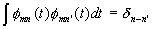
L2(R). This implies the Parseval energy relation holds. And the orthonormal wavelets {j mn(t) } satisfy
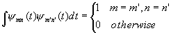 ,
,
which means {j mn(t) } are orthonormal in both
indices, i.e., for the same scale m they are orthonormal in time, and they are also
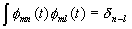
orthonormal across the scales. But the scaling function f (t)
can just satisfy orthonormal condition only within the same scale, i.e.,
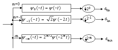
We can image that the wavelet coefficients as being generated by the wavelet filter
bank of following figure. The convolution of f(t) with j m(-t)
is
 where
where 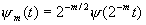
Sampling ym(t) at n2m gives us
- Multiresolution Signal Decomposition
Multiresolution signal analysis provides the vehicle for the links of wavelet transform
and filter banks. In this representation, we express a function fÎ
L2 as a limit of successive approximations corresponds to different solutions.
This smoothing is accomplished by convolution with a low-pass kernel called scaling
function f (t).
A multiresolution analysis consists of a sequence of closed subspaces {Vm |
mÎ Z}of L2(R) which have the following properties:
- containment:
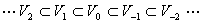
¬ coarser finer®
- completeness:

- Scaling property:

- The basis/frame property:
There exists a scaling function f (t)Î
V0 such that for any mÎ Z, the set
is an orthonormal basis for Vm, i.e.,
- Complement property:
Let Wm be the orthonormal complement of Vm in Vm-1,
i.e.,

Furthermore, let the direct sum of the possibly infinite spaces Wm span L2(R):

we will associate the scaling function f (t) with the space
V0, and the wavelet function j (t) with the space W0.
Define the projection operators Pm and Qm, from L2(R) to
Vm, Wm respectively. The completeness property implies that 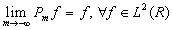 and the containment property implies that as m decreases Pmf
leads to successively approximations of f.
and the containment property implies that as m decreases Pmf
leads to successively approximations of f.
Any function fÎ L2(R) can be approximated by Pm-1f,
its projection to Vm-1. Then it can be express as a sum of projections of Vm
and Wm:
Pm-1f=Pmf+Qmf
Suppose we start with a scaling function f (t), such that
its translation {f (t-n)} span V0. Then V-1
is spanned by {f (2t-n)}. Because of f
(t)Î V0Ì V1,
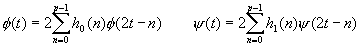
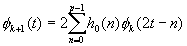
f (t) cab be expressed as:
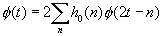
The coefficient set {h0(n)} is the so-called interscale basis coefficients.
The same equation comes to wavelet function j (t):
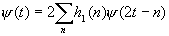
This is the fundamental wavelet equation. We may say later that the h0(n)
and h1(n) will be identified with the low-pass and high-pass branch sample
response of the two-band paraunitary filter bank, respectively.
The above two equations can be used to construct the wavelets:
Because of 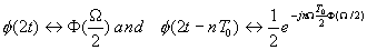
We can have
Now with w =W T0 as a
normalized frequency and H0(ejw ) as the
transform of {h0(n)}:
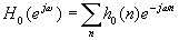
we can get:
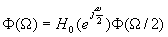
which can be iterated written as:
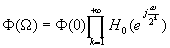
The similar equation comes to wavelet function:

So H0 can be used to construct the wavelet and the scaling functions.
The multiresolution signal decomposition presented above can be used to calculate WT
coefficients, i.e., we can use the PR-QMF filter bank to get WT coefficients. Support that
we have a function fÎ V0, then:

Next, since V0=V1Å W1, we
can express f as the sum of two functions, one lying entirely in space V1 and
another one in the orthogonal complement space W1:

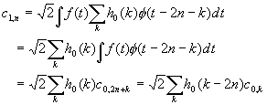
where the scaling coefficients c1,n and the wavelet coefficients d1,n
are given by:

multiply both side of the decomposition equation with f 1,n(t)
then intergrate:
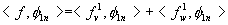
Since fw1(t) is a linear combination of wavelet {j 1k(t) }, each component of which is
orthogonal to f 1n(t), the second inner product is
therefore zero, leaving us with
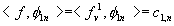
Therefore, we get
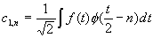
actually from the interscale relationship of the scaling function, we have:
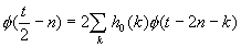
therefore we can represent the new coefficient as:
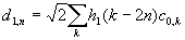
In a similar way we can get
The decomposition of signal can be shown in the following diagram:
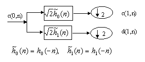
Similarly the signal c(0,n) can be re-construct with c(1,n) and d(1,n):
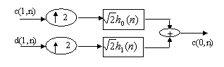
The decomposition of coarser signal component c can be further proceeded as you like.
This is the so-called multiresolution (pyramid) decomposition and reconstitution.
- Two-band Paraunitary PR-QMF and Wavelet Bases
We can get the following equations from the interscale equation and the properties of
wavelet and scaling functions:
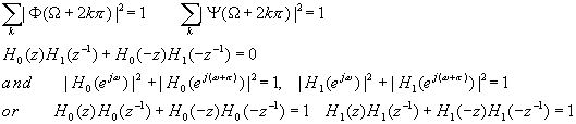
which means that the H0, H1 correspond to low-pass and high-pass
requirement in the 2 channel unitary PR-QMF, respectively.
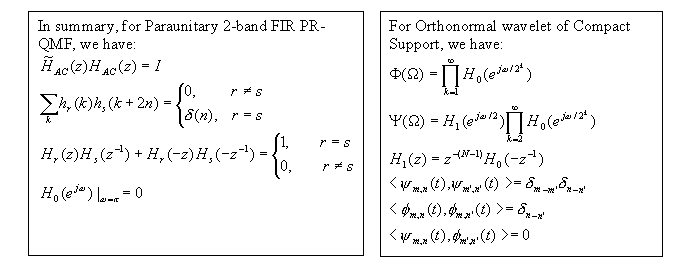
Although there are several wavelets that can be expressed as explicit functions of
time, such as Harr, Shannon, and Gauss wavelet, the wavelets associated with two-scale
equations (interscale functions) are not. Recursions are need to construct them. The
wavelet construction equations are:
Given h0(n) and h1(n), the first step is the generation of f (t) and then j (t) using the following
iteration:
One must notice that Paraunitary PR-QMF can not construct linear phrase FIR banks, that
is to say, following the above multiresolution wavelet decomposition, we can not construct
linear phrase wavelet or scaling functions. To get the linear phrase, we must discard
Paraunitary property of FIR banks, and replace it with binormal FIR banks and wavelets,
i.e., using two multiresolution representations of L2(R).