1. The measure of information

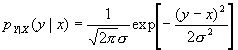
Let {a₁, a₂,…, a_K} be the X sample space and {b₁, b₂,…, b_K} be the Y sample space in an XY joint ensemble with the probability assignment P_XY(a_k,b_j). For example x may be interpreted as being the input letter to a noisy discrete channel and y as being the output. We want a quantitative measure of how much the occurrence of a particular alternative, say b_j, in the Y ensemble tell us about the possibility of some alternative, say a_k, in the X ensemble. In probabilistic terms, the occurrence of y=b_j changes the probability of x=a_k from the a priori probability P_X(a_k) to a posteriori probability P_X|Y(a_k|b_j). The quantitative measure of this can be fundamentally defined as:

The information provided about the event x=a_k by the occurrence of event y=b_j is

The base of the logarithm in this definition determines the numerical scale used to measure information. For base 2 logarithms, the numerical scale of above definition is called the number of bits (binary digits) of information, whereas for natural logarithms, the numerical value is the nats (natural units of information.

It can be seen that from the above definition, the mutual information is a random variable, that is, a numerical function of the elements in the sample spaces. The mean value, which is called the average mutual information and denoted by I(X,Y), is given by

It can be seen that the average mutual information is a function only of the XY ensemble, whereas the random variable mutual information is also a function of particular x and y outcomes. An interesting special case of the mutual information is the case when the occurrence of a given y outcome, say y=b_j, uniquely specifies the outcome to be a given element a_k. In this case P_X|Y(a_k|b_j)=1, and we have

This can be defined as the self-information of the event x=a_k since this is the mutual information required to specify x=a_k. As the mutual information, the self-information is also a random variable. The entropy of the ensemble is defined to be average value of the self-information and is given by:

The bigger H(X) of a source is, the more materials are need to present it. So H(X) may be thought as the uncertainty of a source.

Similarly we can define the conditional self-information of an event x=ak, given the occurrence of y=bj, as

and the conditional entropy as

This can be interpreted as the average information (over x and y) required to specify x after y is known.

There are several important relationships between these definitions:

where H(XY) is defined as XY is a joint ensemble, i.e.,

We also have:

1. with equality iff X and Y are statistically independent.
2. , where K is the size of the ensemble. The equality holds iff all elements are equally probable.
3. Let XYZ be a joint discrete ensemble. Then and with equality iff, conditional on each z, X and Y are statistically independent, i.e., iff

The situation in which I(X;Y|Z)=0 has a interesting interpretation. We can visualize the situation as a pair of channels in cascade as shown in following figure. The X is the input ensemble to the first channel, and Z ensemble is the output of the first channel and at the same time, is the input to the second channel. We assume that the output of the second channel depends statistically only on the input to the second channel, i.e., . Multiply both side of it with P(x|z), we can get I(X;Y|Z)=0.

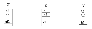
For such a pair of cascaded channels, it is reasonable to expect the average mutual information between X and Y to be no greater than that through either channel separately, i.e., I(X;Z) ³ I(X;Z) and I(Y;Z) ³ I(X;Y). Consequently, we can get H(X|Z) £ H(X|Y), which means that the average uncertainty (entropy) can never decrease as we go further from the input on a sequence of cascaded channels.

1. Coding for discrete source

Consider u_L=(u₁, u₂,…, u_L) to be a sequence of L consecutive letters from a discrete source. Each letter is a selection from the alphabet a₁,…,a_K and thus there are K^L different sequences of length L that might be omitted from the source. Suppose that we wish to encode such sequences into fixed-length code words, i.e., one sequence corresponds to one fixed-length code word. If the code alphabet contains D symbols and if the length of each code word is N, then there are total D^N different code words available. Thus, if we wish to provide a separate code word for each source sequence, we must have:. This means that for fixed-length codes, if we always wish to be able to decode the source sequence from the code word, we need at least logK/logD code letters per source letter.

If we wish to use fewer code letters per source symbol, then we clearly must relax our insistence on always being able to decode the source sequence from the code sequence. In what follows, we shall assign codes words only to a subset of the source sequences of length L. we shall see that by making L sufficient large, we can make the probability of getting a source sequence for which no code word is provided arbitrarily small, and at the same time make the number o code letters per source symbol as close to H(U)/logD as we wish. This can be expressed as the following theorem (Fixed-length Source Coding Theorem):

Theorem: Let a discrete memoryless source have finite entropy H(U) and consider a coding from sequences of L source letters into sequences of N code letters from a code alphabet of size D. Only one source sequence can be assigned to each code sequence and let P_e be the probability of occurrence of a source sequence for which no code word has been assigned. Then for any d >0, if:

, Pe can be made arbitrarily small by making L sufficient large.

Conversely, if , then P_e must become arbitrarily close to 1 as L is made sufficiently large.

In interpreting the theorem, we can think of L being the total number of messages that come out of the source during its lifetime, and think of N as being the total number of code letters that we are willing to use in representing the source. Then we can use any strategy that we wish to code the message sequences and the theorem states that H(U)/logD is the smallest number of code letters per source letter that we can use and still represent the source with high probability.

For variable length code, we also have the following theorem:

Theorem: Given a discrete memoryless source U with entropy H(U), and given a code alphabet of D symbols, it is possible to assign code words to sequence of L source letters in such a way that the prefix condition is satisfied and the average length of the code words per source letter, , satisfies:

. Furthermore, the left-hand side inequality must be satisfied for any uniquely decodable set of code words.

These two theorems are very similar. If we take L arbitrarily large and then apply the law of large numbers to a long string of sequences each of L source letters, we can see the second theorem implies the first part of the first theorem.

2. Discrete Memoryless Channels (DMC)

A transmission channel can be specified in terms of the set of inputs available at the input terminal, the set of output available at the output terminal, and for each input the probability measure on the output events conditional on that input.

The first kind of channel to be considered here is the discrete memoryless channel. This is a channel for which the input and output are each sequences of letters from finite alphabet and for which the output letter at a given time depends statistically only on the corresponding input letter.

Another kind of channel, is the continuous amplitude, discrete-time memoryless channel. Here the input and output are sequences of letters from alphabets consisting of the set of real numbers, and again the output letter at a given time depends statistically only on the input at the corresponding time.

There is another kind of channel, is the continuous time cannel in which the input and output are continuous waveforms. This will be considered latest.

The capacity C of a DMC is defined as the largest average mutual information I(X;Y) that can be transmitted over the channel in one channel use (one channel symbol), maximized over all input probability assignment, i.e.,



We have the following basic theorem, which is used to testify the converse to coding theorem:

Theorem: let U, V be a joint ensemble in which the U and V sample spaces each contain the same M elements, a₁, a₂,…, a_M. Let Pe be the probability that u and v outcomes are different,

, then we have:

, where

This theorem can be interpreted heuristically as follows. The average uncertainty in u given v can be broken into two terms: first, uncertainty as to whether or not an error is made given v; and second, in those cases when a error is made, the uncertainty as to which input was transmitted. The first term is upper bound by H(P_e), and the second is upper bound by P_e times the maximum uncertainty given an error. Since the uncertainty given an error is among M-1 alternatives, the second term is upper bound by P_elog(M-1)

Then we can have the following Converse to the Coding Theorem:

Theorem: Let a discrete stationary source with an alphabet size M and have entropy and produce source letters at a rate of one letter each t s seconds. Let a discrete memoryless channel have capacity C and be used at a rate of one letter (symbol) each t c seconds.let a source sequence of length L be connected to a destination through a sequence of N channel uses (symbols) where N=Lt s/t c. Then for any L, the error probability per source digit, <Pe>, satisfies



The appropriate interpretation of the above theorem is to consider Lt s as the total time over which transmission takes place. Within this total time, the coder can involve fixed-length or variablr-length source coding and block or non-block coding for the channel. No matter what coding or data processing is done, the average error probability per source digit must satisfy above inequality, And is thus bound away from zero if H¥ (U) (the source rate) is greater than C(t s/t c) (the channel capacity per source digit).

3. The noisy-channel coding theorem

Let us assume that binary digits enter the channel encoder at a rate of 1 binary digit eash t s seconds, and that the channel is discrete in time, transmitting one channel digits each t c seconds. We shall restrict our attention to block codes. These are encodes that separate the incoming binary data stream into equal-length sequences of , say, L binary digits each. There are M=2L different binary sequences of length L and the channel encoder provides a code word for each. Each code is a sequence of a fixed number, N, of channel input letters. The number N is called block length of the code, and will be taken as the integer part of L(t s/t c).

The rate of a block code is defined as . The conversion between R (in nats per digit) and the communication engineer’s data rate (in binary digits per second) is thus R=(data rate)´ ln2

We have the following famous Coding Theorem:

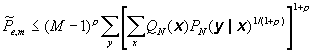
Theorem: Let P_N(y|x) be the transmission probability assignment for sequences of length N³ 1 on a discrete channel. Let Q_N(x) be a arbitrary probability assignment on the channel input sequences (code words) of length N and, for a given number M ³ 2 of code words of block length N, consider the ensemble of codes in which each code word is selected independently with the probability measure Q_N(x). suppose that an arbitrary message m, 1 £ m £ M enter the encoder and the maximum-likelihood decoding strategy is employed. Then the average probability of code word decoding error over this ensemble of code is bound, for any choice of r , 0£ r £ 1, by



The theorem is surprising powerful and general. It applies both to memoryless channels and to channels with memory and can be easily extend to non-discrete channels.

The theorem can be specialized to the case of discrete memoryless channels where

Let Q(k), k=0,1,…,K-1, be an arbitrary probability assignment on the channel input alphabet and let each code word be chosen independently with this probability so that code word probability



then we have:



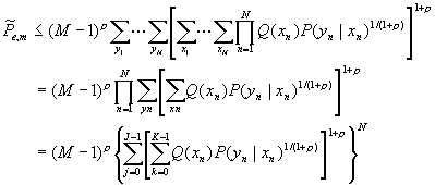
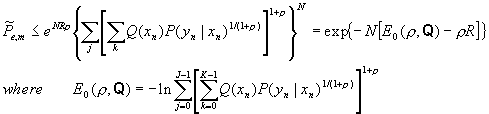
The above inequality bound can be rewrite in a way that will explicitly bring out the exponential dependence of the bound on N for a fixed rate R. recall that R is defined as (lnM)/N. thus M=e^NR, i.e., M varies exponentially with N.

Considering the ensemble of codes above as an ensemble of block code with M-1<e^NR £ M, we have



The above bound is valid for rach message in the code, we can see that the average error probability over the messages, for an arbitrary set of message probability, Pr(m), satisfies



Finally, since r and Q are arbitrary assigned, we can get the tightest bound by choosing r and Q to maximize E₀(r ,Q)- r R. This leads us to define the random coding exponent Er(R) by



Then we have

We can see that the random coding exponent satisfy Er(R)>0 for all R, 0£ R<C, where C is the channel capacity in natural units. Thus we get the important result, by choosing codes words appropriately, the error probability can be made to approach 0 exponentially with increasing block length, N, for any source rate less then channel capacity.

 

4. Momoryless Channels with Discrete Time

In general, a memoryless channel with discrete time is specified by an arbitrary input space X, an arbitrary output space Y, and for each element x in the input space, a conditional probability measure on the output P_Y|X. The channel input is a sequence of letters from the input space, the channel output is a sequence of letters from the output space, and each output letter depends probabilistically only on the correspondingly input letter with the given probability measure P_Y|X.

The general approach to the treatment of these channels can be restrict to the use of a finite set of letters in the input space, say a₁, a₂,…, a_K, and to partition the output space into a finite set of disjoint events, say B₁,…, B_J, whose union is the entire output space. Thin, in principle, we can construct a "quantizer" for which the input each unit of time is the channel output y and for which the output is that event Bj that contains y. The combination of the channel and quantizer is then a discrete memoryless channel with transmission probability P_Y|X(B_j|a_k).

Consider a channel in which the channel output is the sum of the input and independent Gaussian random variable,



It can be shown that if the input is a Gaussian random variable of variance E , then we have



By letting E be arbitrary large, the above mutual information becomes arbritrary large, and by choosing an arbitrary large set of input spaced arbitrary far apart in amplitude, we can see that arbitrary high transmission rate can be achieved with arbitrary low error probability with essentially no coding. If we consider these inputs as samples of a transmitted waveform, however, we see that we are achieving this result through the expenditure of an arbitrary large amount of power. So we have to impose a constraint on the channel input to get physically meaningful and mathematically interesting results. The most useful constraint is the power constraint. We have the following capacity for Gaussian noise channel:

Theorem: Let a discrete-time, memoryless, additive noise channel have Gaussian noise with variance s ² and let the input be constrained by . Then the capacity of the channel is

bits per channel use, i.e., per channel symbol

For non-Gaussian additive noise, the calculation of capacity is a tedious work. The following theorem says that for a given noise variance, Gaussian noise is the worst kind of additive noise from a capacity standpoint.

Theorem: Let a discrete memoryless channel have additive noise z of variance s ² and have the input constraint . Then we have



The item E/s ² is always called (channel symbol) Signal to Noise Ratio, SNR

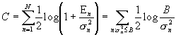
We then consider an important case of a set of parallel, discrete-time, additive Gaussian noise channels. The following theorem finds the capacity of such a parallel combination.

Theorem: Consider a set of N parallel, discrete time, memoryless additive Gaussian noise channels with noise variance s ²₁, s ²₂, …, s ²_N. Let the channel inputs be constrained to satisfy . The channel capacity is achieved by choosing the inputs to be statistically independent, zero mean, Gaussian random variables of variance , where En satisfy



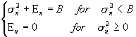
and where B is chosen so that S En=E. The capacity of the parallel combination is



The solution for the input energies to be used on the various channels has the graphical interpretation of following figure.



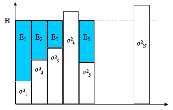
We can think of the total energy E as being a quantity of water to be placed in the reservoir with a irregularly shaped bottem determined by the noise variances. The level to which the water rises is B and the En give the depths of water in the various parts of the reservoir.

5. Waveform channels

There is another kind of channels for which the input and output are functions of time where time will be defined on the continuum rather than at discrete instants.

To evaluate the channel capacity of such channel, we can express any given real or complex waveform as a series expansion of a set of orthonormal waveforms. We then can characterize random waveforms in terms of joint probability distributions over the coefficients in such a series expansion.

Let x(t) be an L² input and y(t) the output from a continuous time channel. Let j ₁(t), j ₂(t),… be a complete set of real orthonormal functions defined over the interval (0,T). then we can represent x(t) over the interval by

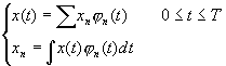
similarly, if q ₁(t), q ₂(t),… is another complete set of orthonormal functions over (0,T), we can represent y(t) by the variables

the set {q n(t)} can be the same as the set {j n(t)}, and such a choice is ofter convenient.

Let x^N and y^N be the sequence x^N=(x₁,…, x_N), y^N=(y₁,…y_N). Then the continuous channel can be described statistically in terms of the joint conditional probability densities p_N(y^N|x^N) given for all N. to avoid the influence of x(t) for t<0, we assume x(t)=0 for t<0. We also assume that the input ensemble can be described by a joint probability density q^N(x^N) for all N. the mutual information between x(t) and y(t) for 0£ t £ T, if it exists, is then given by:

where

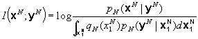
And the average mutual information between input and output over the interval (0,T) is given, if it exists, by

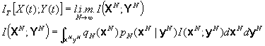
Please note that is implicitly a function both of T and q^N(x^N). The capacity of the channel, per unit time, is defined by

where the supermum is over all input probability distributions consistent with the input constraints on the channel. The quantity in the brackets above is the maximum mutual information that can be transmitted in time T.

Please note that the definition here is slightly different with those defined previously. The C here is the average mutual information (bits) per second, and those are bits per channel use, i.e., per channel symbol.

We have the following famous theorem:

Theorem: Let the output of a continuous time channel be given by the sum of input and white Gaussian noise of spectral density No/2. And let the input be power constrained to a power S. then the capacity of the channel per unit time is given by

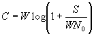, where W is the bandwidth of the channel.

There are some important conclusions from above theorem. The equation can be drawn in the following figure:

As W® ¥ , we can see that the C ® (S/N₀)loge.

We can establish an interesting bound on the transmission rate of information. Suppose that the actual information rate is R bps. From above theorem, we have R £ Wlog(1+S/N₀W). This can be expressed in terms of energy per source bit, Eb=S/R, as

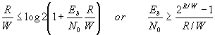
For the case of infinite bandwidth, this becomes

This equation gives the lower bound on the amount of energy per transmitted bit that is required for reliable communications through the additive white Gaussian noise channel. If the signal-to-noise ratio per bit is less then –1.6 dB, it is not possible to transmit error free no matter how much bandwidth is used.

For the channel shown in following figure with a power constraint S and with T0=T, assume that H₁(f)²/N(f) is bounded and integrable, and that either F N(f)df < ¥ or that N(f) is white. Then the capacity of the channel is given parametrically by

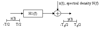
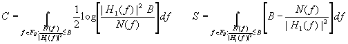
The power spectral density for the input ensemble that achieves capacity is given as:

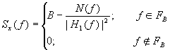
F_B is the range of f for which N(f)/|H₁(f)|^2£ B, and B is the solution to above right-side equation.

The theorem is called water-pulling theorem and can be interpreted as following figure:

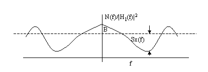
we can think of N(f)/|H1(f)|² as being the bottom of a container of unit depth and of pouring in an amount of water S. Assuming the region to be connected, we see that the water (power) will distributed itself in such a way to achieve capacity. The capacity is proportional to the integral of the log of the ration of the water level B to the container bottom N(f)/|H₁(f)|².