Transmission Lines
For some people, transmission line may just simply be a piece of wire. But in RF system, any cable or wire with physical length greater than the wavelength of a signal passing through this wire is called transmission line.
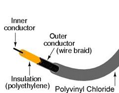
There are various types of transmission lines such as coaxial cables, strip lines, microstrips, waveguides, etc… The most common transmission line used in RF transmission is the coaxial cable or the coax.
An example of coaxial cable
High frequency pulses tend to attenuate when they are passed through any cable. The amount of attenuation depends on the data rate, transmission distance, and the cable’s electrical characteristics.
Electrically, we can define transmission line as a network of resistors, inductors and capacitors as shown.

An example of one unit length of transmission line
Transmission line matching (Impedance matching)
The characteristic impedance - the ratio of a pair of voltage and current waves at any point on that transmission line in the absence of reflections - may or may not be constant. Characteristic impedance (ZO) can be defined as:

It is very important to transfer radio frequency energy from a generator to a load through transmission lines with zero or minimum power loss. To achieve this, the source and the load impedances have to be matched. And the transmission line between them should have equal characteristic impedance as well (usually 50 Ω for RF transmission).
Impedance mismatch in the transmission line will cause some of the signal power reaching to the load to be reflected back and produce standing wave.
We can measure the amount of reflected power by reflection coefficient (Γ)

The coefficient has to be as small as possible. The ideal value is zero when the load impedance is the same as the characteristic impedance.
Now, we know that it’s very important to have matched impedance in RF system. To ensure this happen, we can:
 ZS=ZL*
Circuit representation of ZS and ZL configuration
Impedance matching networks
The purpose of impedance matching network is to conjugate match the source and the load. And when the load impedance is the conjugate of the source impedance, maximum power is transferred.
Two-element impedance matching networks will be discussed here. There are eight possible LC, LL and CC combinations that can be used in two element impedance matching networks.
Four combinations for LL and CC networks
Four combinations for LC networks
The above eight networks can be approached by mathematical manipulation or by Smith chart. Smith Chart will be discussed here as it is easier to understand.
Smith Chart
Smith chart is basically a combination of circles and arcs to represent rectangular form of impedance and admittance at a specific frequency. By using smith chart, we can leave behind all the complications of using mathematical equations. Basically, we have three types of Smith chart; Z, Y and ZY smith chart.
Z smith chart or impedance smith chart shows rectangular form of impedance.
The centre line shows you the resistance value.
Y smith chart or admittance smith chart shows rectangular form of admittance (Y=1/Z)
ZY smith chart or admittance smith chart is the superimposition of X and Y smith chart.
Let us try out one example to understand more about Smith Chart.
But first, we need to know that to use smith chart, we must normalise the impedance value.
ZN=Z/ZO ZN=normalized impedance
ZS=the impedance that needs to be normalized
ZO=characteristic impedance (usually 50 ohm for RF transmission)
YN=1/ZN
Say, we have to design an L-matching network for ZS=25-j15, ZL=100-j25 at 60 MHz. Follow the steps in the following animation.
We can verify our calculation, by checking if the input and output impedances (Zin and Zout) are complex conjugates of the ZS and ZL.
From the circuit, we can derive these two equations,
Zin = (j.ω.L) + [ZL || ![]() ] eq(1)
] eq(1)
Zout = (ZS + j.ω.L) || [![]() ] eq(2)
] eq(2)
Solving eq(1),
Zin = (j.ω.L) + [ZL || ![]() ]
]
= [j (2π x 60 x 106 x 159 x 10-9)] + [(100-j25) || (![]() )]
)]
= j60 + [(100 – j25) || (-j68.5)]
≈ 25 + j15 (verified that Zin is the complex conjugate of ZS)
Solving eq (2),
Zout = (ZS + j.ω.L) || [![]() ]
]
= [25-j15 + j (2π x 60 x 106 x 159 x 10-9)] || [![]() ]
]
= [25 – j45] || [-j68.5]
≈ 100 + j25 (verified that Zout is the complex conjugate of ZL)
You can also try and see what happens when you add a parallel inductor first then a series capacitor. Check below for solution:

References List